
Dev Training: Big O Notation
You don’t have to be a computer scientist to write the most efficient code, but knowing good algorithms from bad ones certainly helps.
Most developers aren’t born mathematicians. And that’s fine. Software developers generally need to learn a lot of other things like language syntax, common pitfalls, and structural design. They can use the tools created for them to produce some pretty amazing applications. But because computers and software come from mathematics, developers often bump into it.
And that’s not always a bad thing. Sometimes, a little knowledge can help.
Take writing algorithms, for example.
All developers can put together a program that does something. It has a start, takes some data, does something with it, and eventually ends. A basic program with a simple algorithm is easy. But some programs aren’t simple. Some data sets aren’t small. Manipulating large tables of data sometimes requires a little more thought, and that can result in a more complicated algorithm.
Algorithm Design
There are lots of different approaches to designing algorithms. You can take a Greedy approach, a divide-and-conquer style attack, a brute-force search or even an optimized dynamic style. Each is best suited to a different kind of problem. Picking the right approach can be difficult.
To check if an algorithm is best suited to a problem, it’s useful to have tools or ways of describing and comparing characteristics like performance or complexity. This is where Big O notation comes in useful.
Big O Notation
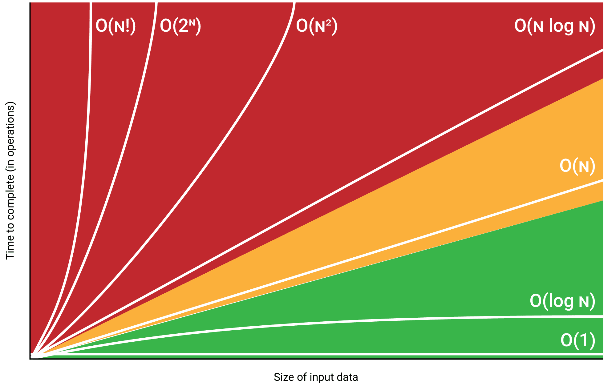
Big O Notation is a way of describing how well an algorithm will scale as the size of its input increases. Understanding it helps you to design better algorithms and gives you some things to be aware of.
It’s a mathematical way of writing about how a function’s time to complete changes as the size of its input data changes. As input data gets larger, the increase in time is called the growth rate, and Big O notation describes that growth rate.
It’s also used to describe how the space needed at any point in an algorithm grows as the input grows, but for this article, I’ll focus only on time complexity.
It’s worth noting that because data can vary, how long it takes a function to do its job can vary too. A function that searches an array may either find what it’s looking for immediately or search the whole array before being successful. Big O notation always describes the worst-case scenario.
Each level of complexity described by Big O notation also has a rating of how well it scales as input sizes grow: some well, some terribly. But if a level of complexity scales badly, that doesn’t mean it should always be avoided. Some problems have solutions that don’t scale well. When faced with a solution that doesn’t scale well, it’s important to be aware of what size of input the algorithm can comfortably manage and keep the input data below that limit.
In this article, I cover 8 of the most commonly used notations. I’ll explain how each is defined, along with its name and some common algorithms or data structure operations that can be described as using Big O Notation. I’ll show some code that serves as a good example and, where possible, point out some design suggestions each one highlights.
O(1)
Algorithms or functions described as O(1) have no growth rate, meaning they don’t take longer the larger their input gets. Their growth rate is classed as constant. Accessing an array is described as O(1) because it doesn’t matter how large the array is, it will always take the same time to get an element.
def get_first_item(items):
    return items[0]
O(n)
Functions described as O(n) have a linear growth rate. As the size of their input grows, the time to complete grows at the same pace. Any algorithm that has to go through an entire data set once before completing is likely to be classed as O(n). Searching for a value in an array is O(n), as potentially the whole array must be visited to find a value. A linear growth rate is considered to be good.
def find_user(usernames, user):
    for username in usernames:
        if username == user:
            return True
    return False
O(n^2)
If a function loops over a dataset and with each item also does something with every other item, you’re looking at O(n^2), or quadratic. Because of how fast the time to complete can grow, this isn’t considered efficient, and is only suitable for smaller sized inputs. A selection sort algorithm is a good example of an O(n^2) function.
This level of complexity suggests that if you find an algorithm which analyses an array at the same times as traversing it, remember that there will be a limit on the size of inputs it can manage well.
def make_pairs(items):
    pairs = []

    for i in range(len(items)):
        for j in range(len(items)):
            pairs.append(items[i] + ", " + items[j])

    return pairs
O(n^c)
Functions which have a growth rate of O(n^c) are known as polynomial and are considered to scale terribly. O(n^c) is like O(n^2) except that not only does it loop through data and do something with every other item, but it does it more than once (C times).
This can create a phenomenal rate of growth. As the size of the input grows, the time it takes to complete heads skyward. Assuming C = 3, a 100-element list would require 1,000,000 passes; a 1000-element list 1,000,000,000 passes.
def make_triplets(items):
    triplets = []

    for i in range(len(items)):
        for j in range(len(items)):
            for k in range(len(items)):
                triplets.append(items[i] + ", " + items[j] + ", " + items[k])

    return triplets
O(2^n)
Another one belonging to the scales badly group is O(2^n) known as exponential. It describes an algorithm whose time to complete doubles with each single extra item in its input. It’s nearly the worst level of complexity out of the 8. An example of this is a basic function for calculating Fibonacci numbers without optimizations.
def calculate_fibonacci(number):
    if number <= 1:
        return number

    return calculate_fibonacci(number - 2) + calculate_fibonacci(number - 1)
O(log n)
O(log n) is considered the golden child of Big O notation. Algorithms defined as O(log n) have a logarithmic growth rate and excluding O(1) are considered to be the best growth rate to achieve. The time taken to complete only increases each time the input size doubles, which means as the input size grows substantially the algorithm’s time taken to complete only increases a little.
It does this by being intelligent with how it treats the data. O(log n) algorithms try not to use the complete input data and instead try to reduce the size of the problem with each iteration.
Take a binary search algorithm which searches a sorted array. It begins by going to the middle of the array and deciding to go up or down the array. In one iteration, it instantly knows it can ignore half of the array.
This highlights that when dealing with a large amount of data, it’s worth considering how you can organize the data so that you can make intelligent assumptions. Finding a way of discounting data as you traverse will help create an algorithm that scales well.
def demonstrate_log_n(items):
    i = len(items)
    while i > 0:
        print("Position " + str(i) + " visited.")
        i //= 2
O(n log n)
Algorithms defined as O(n log n) have a similar growth rate to O(n) except that it’s multiplied by the log of the number of items in the input, which makes it a little worse. Unfortunately, this makes it not so good. Some sorting algorithms like mergesort or heapsort can be defined as O(n log n). Imagine an algorithm that loops through an array and for each iteration, like O(n^2), it does something with other items of the array. But unlike O(n^2), it only does something with a selection of the array. The algorithm has some way of making an intelligent choice about which items to look at.
This emphasizes that if you have an algorithm that feels like it’s O(n^2), it’s always worth remembering that just because you have to traverse the whole data set once, doesn’t mean a further efficiency can’t be found in a later step. Always try to keep looking for ways to reduce the size of the problem.
def demonstrate_n_log_n(items):
    for j in range(len(items)):
        i = len(items)
        while i > 0:
            print("Position " + str(j) + ", " + str(i) + " visited.")
            i //= 2
Summary
Hopefully, this brief overview will help you understand Big O Notation. Not only is it a useful tool to help describe algorithms, but it also helps when deciding which data structure or sorting algorithm to choose.
Resources
Here are some great links to learn more about Big O Notation:
Big O Notation on Wikipedia
Table of Common Time Complexities on Wikipedia
Big O Cheat Sheet